The Eigen* Refresher
Disclaimer: This post assumes a basic familiarity with linear algebra topics.
This is the first of the 2 blog posts on topics of eigenvectors and how they relate to the technique of PCA. In this post, we’ll revisit some basics of eigenvectors and their interpretation.
Matrices as Linear Transformation Functions
To be able to interpret eigenvectors geometrically, we start with the interpretation of a $n \times n$ matrix. Let’s take the following example:
\[A ~=~ \begin{bmatrix} 3 & 1\\ 0 & 2 \end{bmatrix}\]
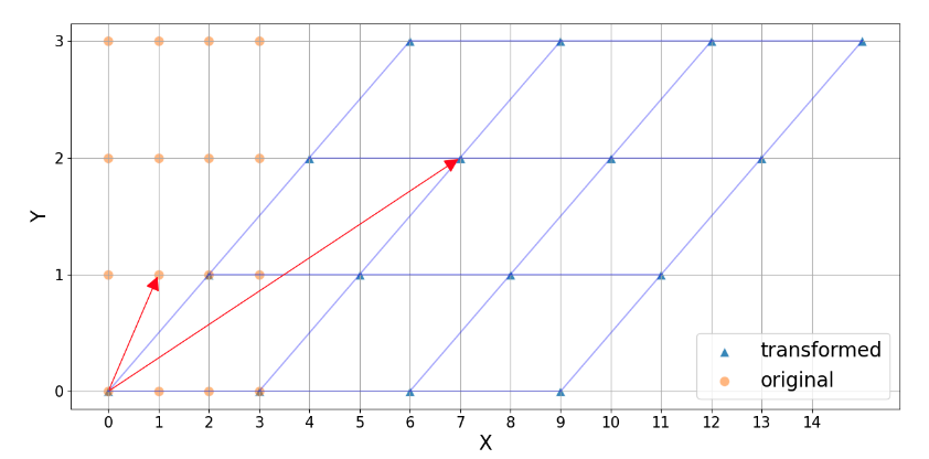
Multiplying this matrix with any point $\mathbf{x} = (x_1, x_2)$ gives us the position of this point in the space defined by the transformation A. Algebraically, the point $\mathbf{x}$ is mapped to $(3x_1 + x_2, 2x_2)$.
\[\begin{bmatrix} 3 & 1\\ 0 & 2 \end{bmatrix} \times \begin{bmatrix} x_1\\ x_2 \end{bmatrix} ~=~ \begin{bmatrix} 3x_1 + x_2\\ 2x_2 \end{bmatrix}\]Note, how the transformation affects the vector $\mathbf{x} = (1, 1)$, shown by red arrows.
Geometric Interpretation of Eigenvectors and Eigenvalues
It’s certainly not obvious, but there are some special vectors that are not affected by this transformation. For example, $(1, 0)$. This vector has the same direction before and after the transformation, although it gets scaled by a factor of 3. This scaling factor is the eigenvalue associated with that vector.
\[\begin{bmatrix} 3 & 1\\ 0 & 2 \end{bmatrix} \times \begin{bmatrix} 1\\ 0 \end{bmatrix} ~=~ 3\begin{bmatrix} 1\\ 0 \end{bmatrix}\]If we were to do some math, we can find the other (rather sneaky) eigenvector corresponding to the $y = -x$ line:
\[x_2 = \begin{bmatrix} -1/\sqrt{2} \\ 1/\sqrt{2} \end{bmatrix}\]When I first learned about eigenvectors I had a hard time understanding the significance and the need to introduce such abstract concepts. I won’t claim I understand it completely now, but I do have a new appreciation for how cool these ideas actually are. This post is a way to share some of that understanding.
So what are eigenvectors really? They are vectors characteristic to a given matrix (transformation) and together they define the transformation space just like X and Y axes in a 2D coordinate system do.
What to do with Eigenvectors?
Let me share a very interesting property to demonstrate a simple use for the eigenvectors. Suppose $A$ is an $n \times n$ matrix with n linearly independent eigenvectors $v_1, v_2, \cdots v_n$. If $C = [v_1, v_2, \cdots v_n]$, then $C^{-1}AC$ is a diagonal matrix with the diagonal entries corresponding to the eigenvalues of A, i.e.
\[C^{-1}AC = \begin{bmatrix} \lambda_{1} & & \\ & \ddots & \\ & & \lambda_{n} \end{bmatrix}\]Almost magical, isn’t it? Although the algebraic proof is straightforward, I find the geometric interpretation a lot better. $C^{-1}AC$ is a composition of 3 transformations applied successively from right to left. The first transformation $C$ maps us to the eigenspace. The second, $A$, performs the core transformation; note that the direction of the eigenvectors remain unchanged after this. And finally, we revert the first transformation, $C^{-1}$, to bring us back to the “standard” space. This composition, therefore, captures how the transformation looks like in the eigenspace. And indeed, in the eigenspace, the core transformation has only a scaling effect on the coordinate axes and therefore the result is a diagonal matrix.
One practical application of this is in computing $A^k$. For our example above, instead of actually performing $k$ successive matrix multiplications, we can do the following:
\[A^k = C \begin{bmatrix} \lambda^{k}_{1} & & \\ & \ddots & \\ & & \lambda^{k}_{n} \end{bmatrix} C^{-1}\]A lot cleaner, right?
Eigenvectors for Data Science
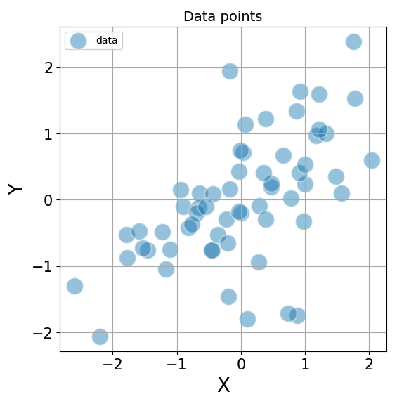
Eigenvectors have a much simpler interpretation when looking at distributions of data points. For example, consider the scatterplot below of two variables X and Y.

It is clear that there is a positive covariance between the X and Y variables. When computed exactly, can be represented by the following covariance matrix
\[cov(X, Y) = \begin{bmatrix} 1.09 & 0.57\\ 0.57 & 0.89 \end{bmatrix}\]It is easy to imagine computations on this generic (symmetric) matrix quickly becoming cumbersome. It would be so much better if we could work with diagonal matrices instead. This is exactly what we’ll do using the eigenvectors of this matrix.
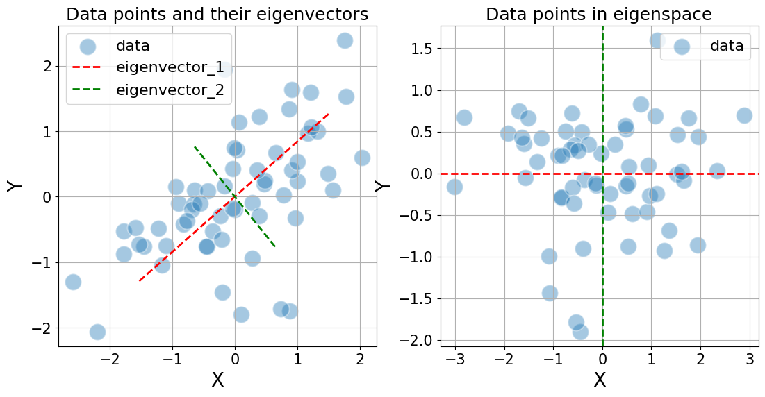
On a side note: Matrices like the covariance matrix come with some especially nice properties on their eigenvectors and eigenvalues. For example, the eigenvalues are always positive and correspond to the variance in the direction of the eigenvector. Furthermore, they are guaranteed to be orthogonal to one another. This is not obvious but goes beyond the scope of this post. Nevetheless, this property allows us to simplify the representation of the data by decorrelating the X and Y axes. See the figure below. We’ll come back to this property and how this decorrelation can be helpful in the next post, when we discuss PCA.

The covariance matrix of the data distribution seen this way is just the diagonal matrix with the diagonal entries corresponding to the variance along the eigenvectors: \(cov^{eigen}(X, Y) = \begin{bmatrix} 1.57 & 0\\ 0 & 0.41 \end{bmatrix}\)
