Better Pricing: Part 2

This post is a continuation of the previous post in the series “Better Pricing”. Last time, I introduced the basic set-up of the problem at hand and the constraint we shall be using. And the objective? Maximizing revenue of course! But we shall go about it in a slightly different way by maximizing the following function:

\[\newcommand{\bm}[1]{\boldsymbol{#1}} \newcommand{\norm}[1]{\left\lVert#1\right\rVert} \newcommand{\p}{\bm{p}} \newcommand{\x}{\bm{x}} \mathcal{L}(\p) ~=~ \p \cdot \x ~-~ \lambda \norm{\p - \p^{old}}^2\\\]

Given this function, we can compute the new optimal price as follows:

\[\DeclareMathOperator*{\argmax}{arg\,max} \norm{\p}^{new} ~=~ \argmax\limits_{\p} \mathcal{L}(\p)\\[8pt] ~~~~s.t.~~ \norm{\p^{new}} ~\leq~ 1.05 \cdot \norm{\p^{old}}\\\]

Toy Example

For purposes of illustration, let’s consider a simplified (discrete) version of the problem, where WoG can be either 0 or 1 (representing two different demand scenarios).

Demand and Prices for different WoG scenarios

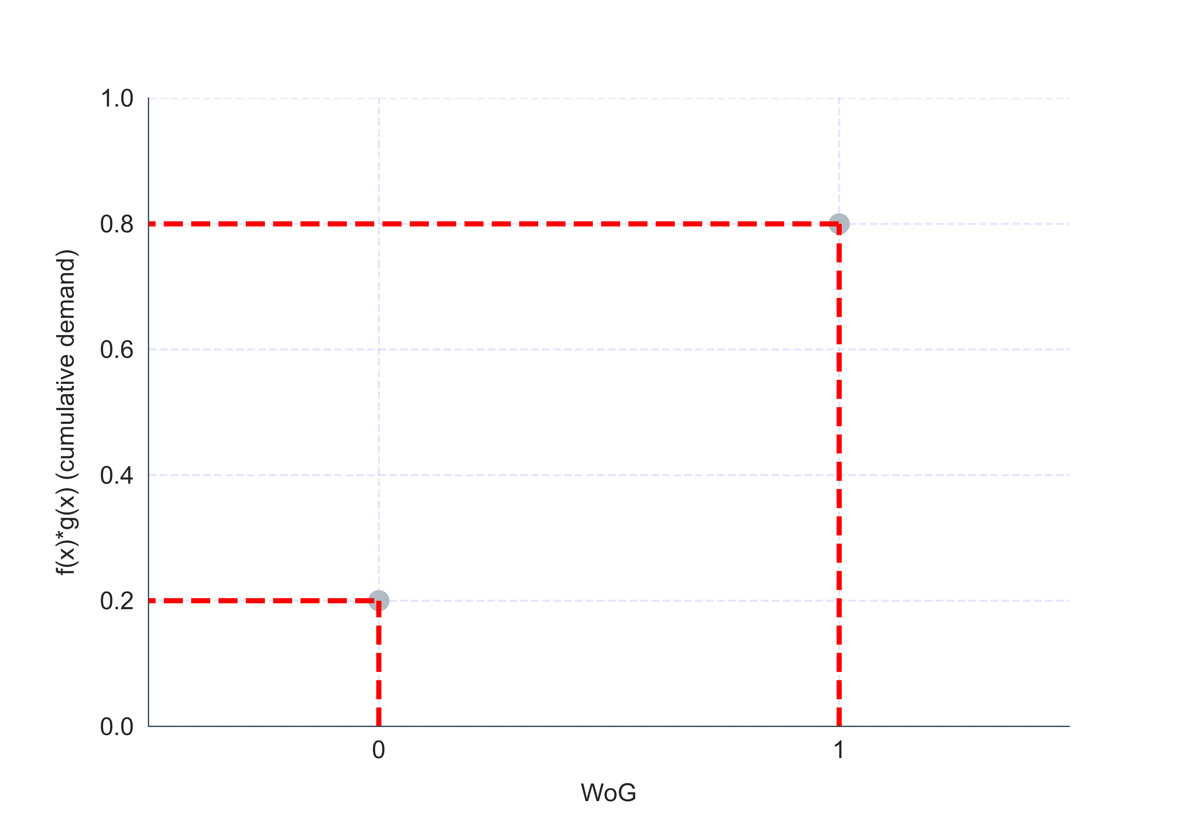
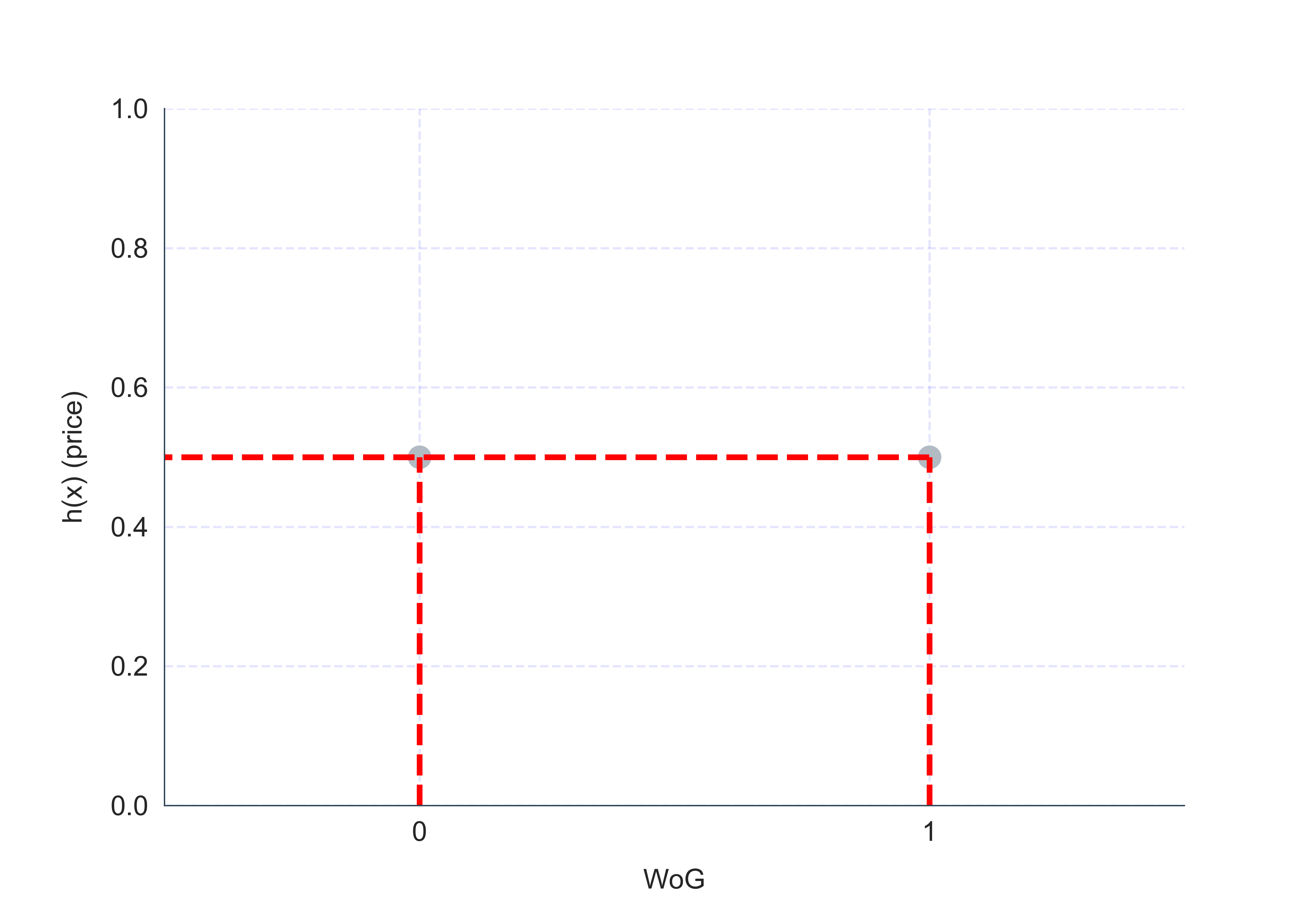
Let’s first visualize the objective function and the solution space. Darker shades of green correspond to smaller numbers.

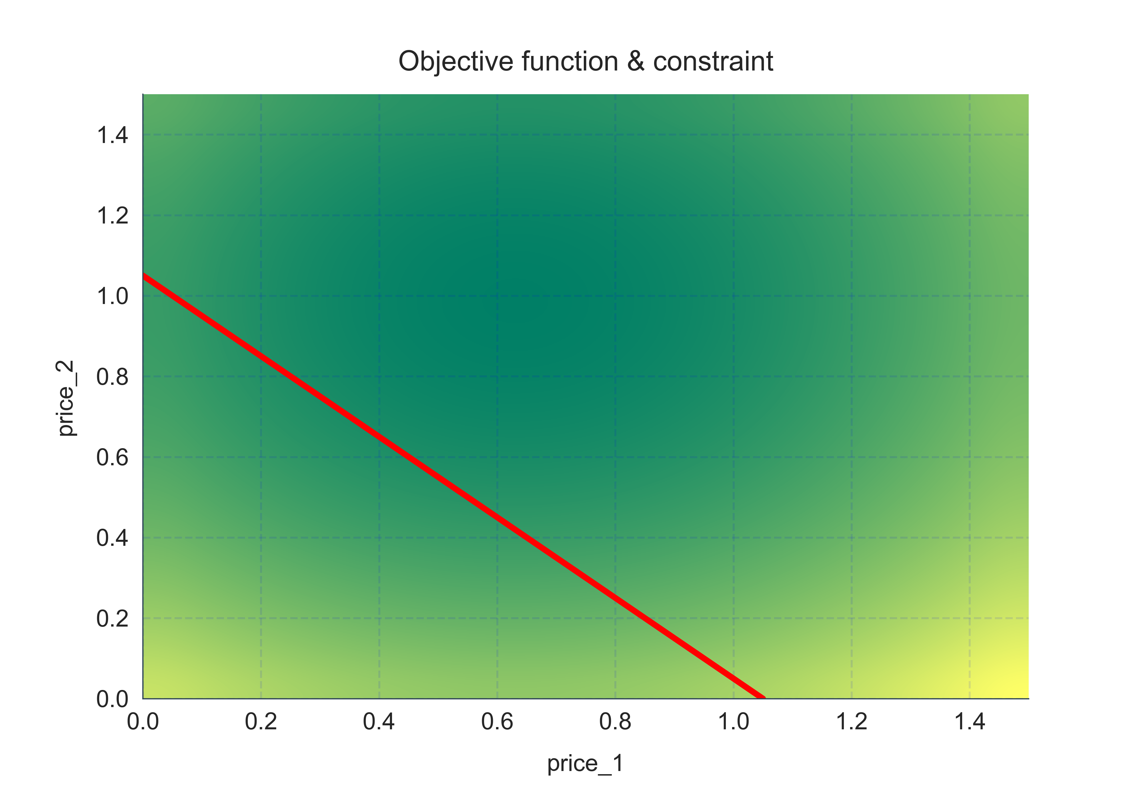
Luckily for us, the objective function is quadratic with linear constraints. This will help us with faster computation. The code snippet used to find optimal prices is as follows:

Let’s see what the new prices are:

Prices after Optimization

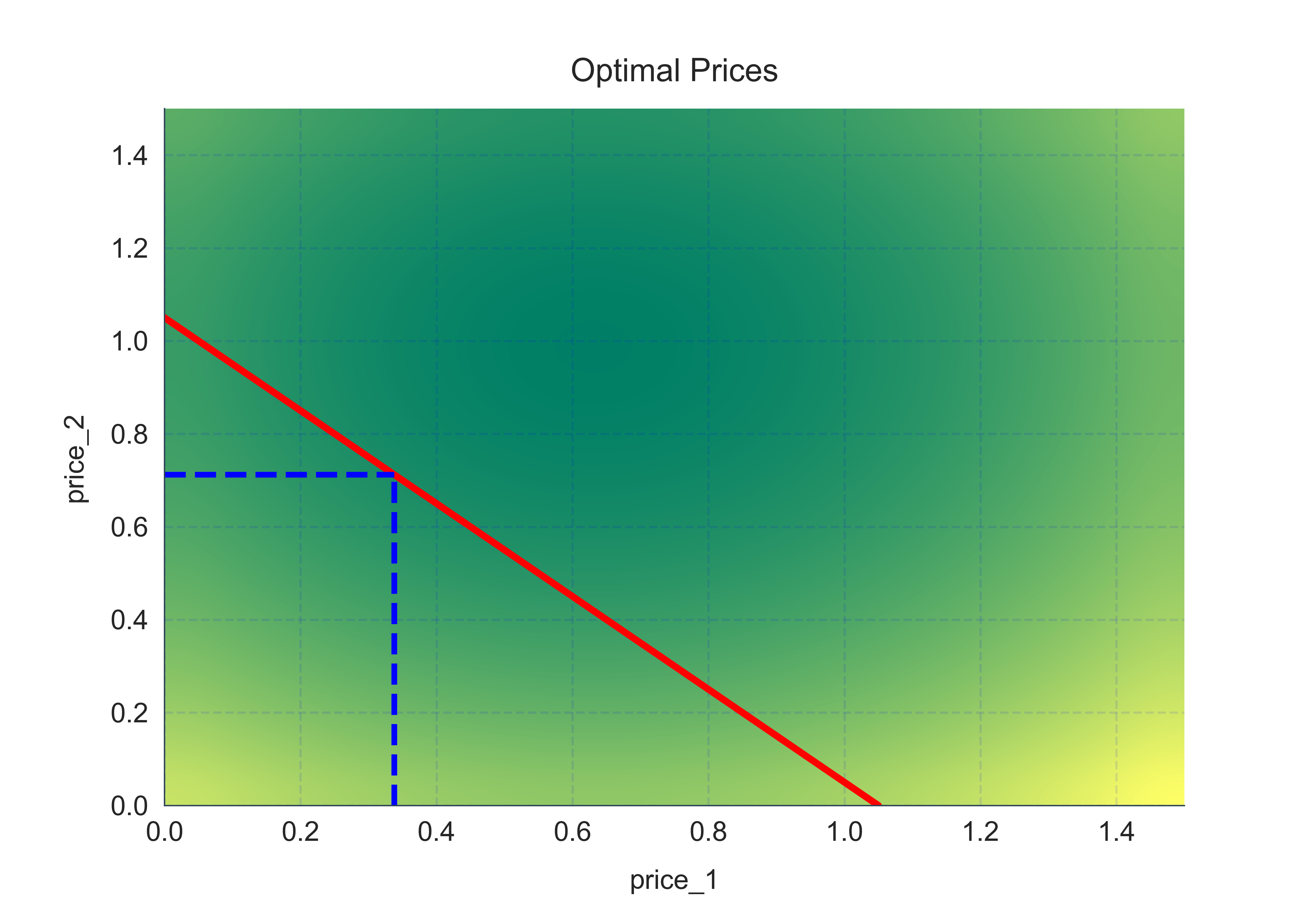
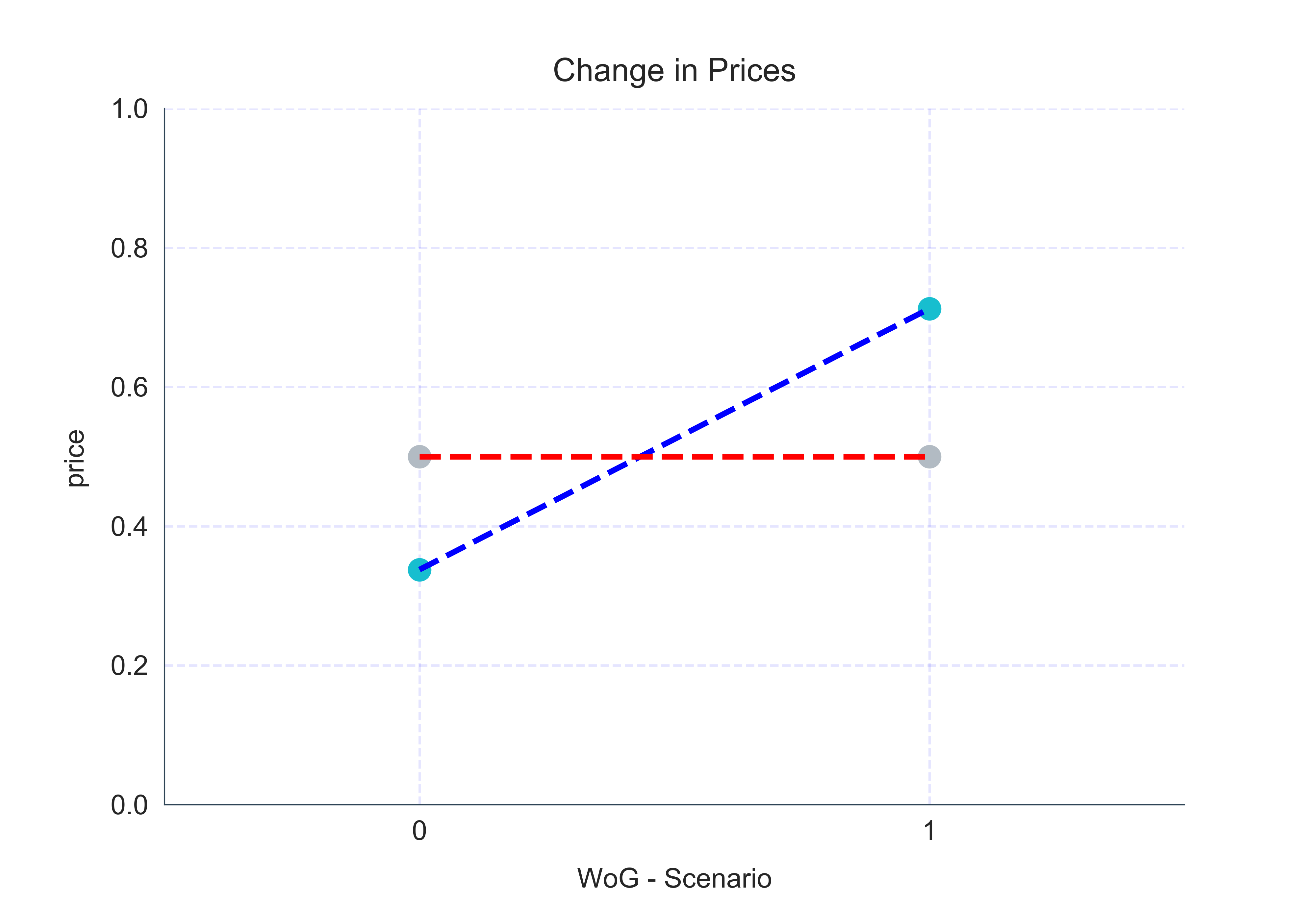
This seems to makes sense: for the low demand scenario (WoG=0), prices have decreased whereas for the high demand scenario (WoG=1) prices have increased. I should point out a couple of things at this point:

1. The optimal hyperparameter $\lambda$, responsible for penalizing changes in prices, in our basic model, cannot be determined in a methodical way. For this example, I manually tried different values to see which ones make sense.
2. Our model does not assume changes in demand on changes in prices. But since the price changes are expected to be rather small, I think the assumption is justified.

Let’s try out a pricing policy with 10 unique price points and how the prices change. The only thing we need to change in the code above is p_old and x_old:

p_old = np.array([0.4]*5 + [0.6]*5)
x_old = np.array(np.linspace(0.2, 0.8, 10))

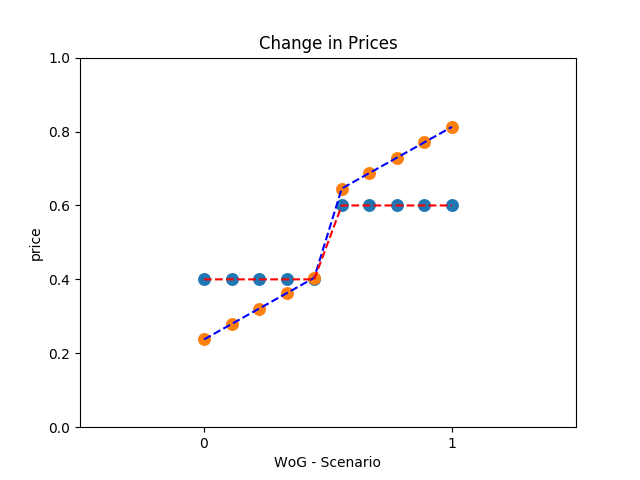
That’s all for now folks. Hope you found the idea interesting!