Exponentiated Gradient for Online Regression
Till now I have worked on problems involving online optimization but in a very abstract sense and mostly along the lines of regret minimization algorithms. Now, I am trying to pursue similar questions but in the context of standard machine learning problems, like regression and classification. It’s both fortunate and unfortunate at the same time that there is already a humongous amount of work done in this field. I am not quite sure which of the works have been most influential in this field, so I am just going to look for some well-cited papers in the coming weeks.
The first one I am going to be looking at is: Exponentiated gradient versus gradient descent for linear predictors and has been cited a staggering 793 times, as of today. There are plenty of things that the authors are doing in this paper (actually, a few too many in my opinion) but in this post, I am focusing on one particular algorithm called EG± and is essentially a variant of the exponential gradient algorithm widely used in Experts problem. I intend this post to be focusing on high-level details (the big picture) while the theoretical analysis is pushed to separate pdf notes.
Dataset: For purposes of experimentation, I am using house pricing dataset from Kaggle. The original dataset has 80 features which I am trimming to 36 (essentially just choosing the numeric data). Out-of-the-box linear regression still works pretty well with the R2 value of around 0.85. Anyhow, the point of the experiment is to see how close our online algorithm comes to the one using batch data. So we’re good. As an aside, I should point out that we are dealing with linear regression here, therefore the hypothesis space is the set of all linear functions.
So, the general idea is as follows: In each round, we choose a weight vector that serves as the hypothesis of the learner and based on this hypothesis the learner predicts a value $\hat{y}_t = w_t \cdot x_t$. Based on this prediction, the learner incurs a loss
$L(y_t, \hat{y}_t) = ( y_t - \hat{y}_t )^2$
The goal of the learner is to update the hypothesis in an online manner such that the cumulative loss incurred is minimized. Of course, one may ask what’s so special about squared loss, and honestly, I am myself not sure, except that it allows one to give good learning bounds.

A couple of comments are in order here:
- eta and U are parameters the learner get to choose. How to set them currently is something we see in the analysis.
- More importantly, note the difference from standard EG algorithm. In EG algorithm, the weights are all positive and always sum to one. Just think about it, this restriction indeed limits the expressive power of our hypothesis. To allow for a more general hypothesis, EGPM chooses two weights for each feature component that allows for both positive and negative coefficients.
- In spite of this modification, the sum of all (positive and negative) weights is required to be U. Therefore, it becomes crucial to choose a good value for U. This also happens to be one of its major drawbacks.
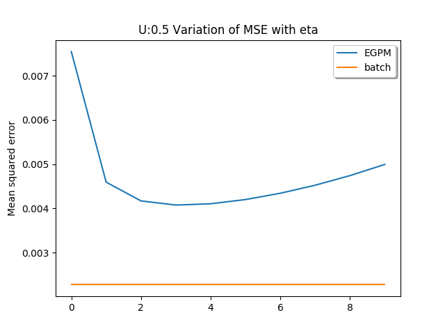
Okay, so let’s see how this really works. After this, we shall focus on a formal analysis. The code used is available on Github. One of the first problems, with implementing this algorithm is exactly what choice of eta and U to use. As we shall see later, without much prior information, this is essentially a guessing game. As an aside, for computational reasons, I have scaled all features to lie in [0, 1] and hence the loss function is also correspondingly scaled down.
In the first experiment, I am comparing the performance of our algorithm with standard linear regression and the curve below represents the mean squared error for different values of step sizes. Given the fact that EGPM starts out with no information at all, I think (for the best value of eta), the algorithm works pretty well! (Of course, I had to try like a hundred times to find the range where it works the best)

Out of curiosity, I tried comparing the performance to degree 2 polynomial as well. The interesting part is, that such a transformation results in ~740 features (considering every possible degree 2 monomial). I was assuming that with so many features, EGPM is bound to perform poorly (since the dataset contains only ~1400 instances). Well, surprise, surprise! It still works pretty well!

I personally think this is a pretty awesome performance. Although of course, it has a host of issues to it but to be fair this was published in 1997 and by all means, online learning was in its nascent stages. This is also seen the proof techniques which are very specific and brittle to changes in loss functions. This work was anyhow quickly overshadowed by the then-pioneering work by Cesa-Bianchi in 99, “Analysis of Two Gradient-Based Algorithms for On-Line Regression” where the results were greatly generalized.
